Basics of Machine Learning, the Multi-Layer Perceptron

This first post will guide you through the basic concept of DNNs using the Multi-Layer Perceptron (MLP) as the explanation baseline. MLP’s simplicity makes it easier to understand the structure and elementary processes within Artificial Neural Networks (ANN) and the definitions here can be extrapolated to more complex DNNs. This post does not intend to provide an exhaustive explanation of the training and optimisation of processes but to introduce some key ideas.

The Multi-layer Perceptron (MLP) was one of the first ANNs to appear in the machine learning community. It is an extension of the Perceptron developed by Rosenblatt in 1958. This kind of network, in theory, can “learn” to approximate any kind of linear or non-linear functions. Thereupon, we will dip into the MLP structure to understand how it computes its outputs.

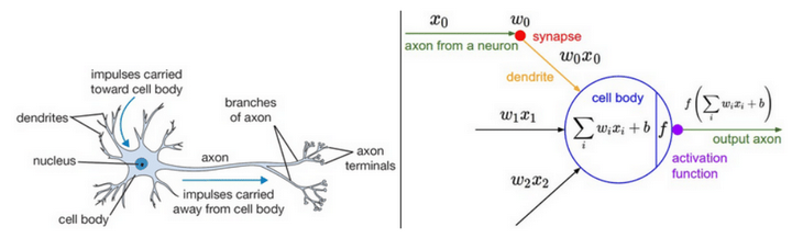
The building block of the MLP is the Perceptron referred to as an artificial neuron. It is inspired by biological neurons, sharing some similarities as depicted in in the header image. It aggregates information from different inputs (dendrites) and generates a single output (axon) that is triggered using an activation function.

(1)

The equation describes how the Perceptron calculates its output. The values from the different inputs are aggregated by performing a weighted sum across all inputs multiplied by some weights and adding a bias term . Therefore, a single Perceptron can approximate linear functions. It is worth noting that the bias term allows the Perceptron to learn functions that don’t necessarily have to pass through the origin. As the reader might have noticed, this is the same equation as a logistic regression where the weights play the same role as the coefficient in the regression.

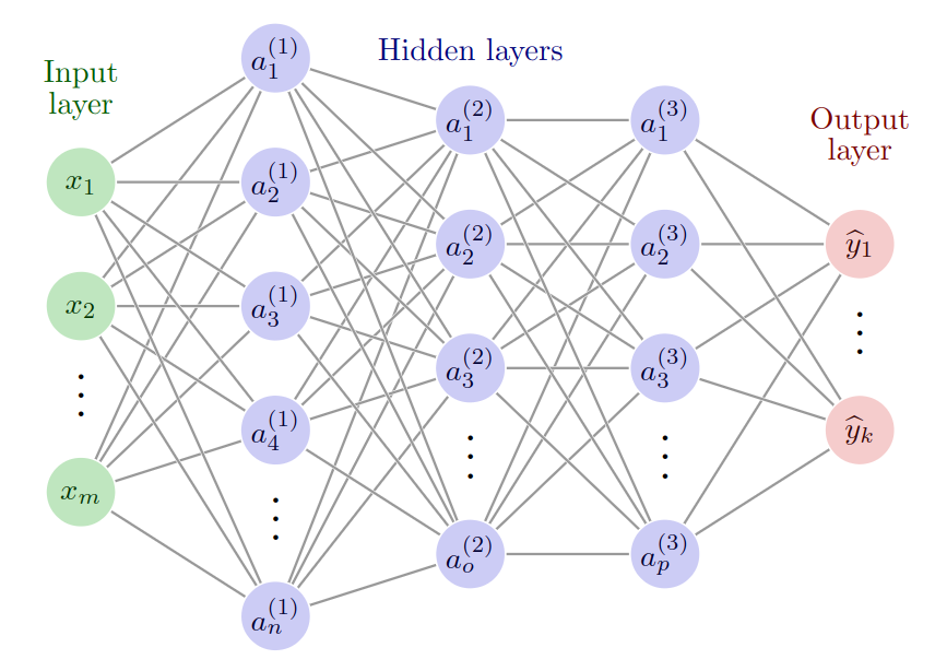
Fig. 1 Multi-Layer Perceptron scheme.

Although the Perceptron by itself is a good approximator for simple linear functions, the real power of the MLP comes from the connection in layers of many of these neurons forming a network. Moreover, the result of Eq. 1 is passed through a non-linear operation , also called activation function, that modules the intensity and range of the values at the output, thereby enabling the MLP to approximate non-linear functions. Further information on these activation functions and the most commonly employed variants can be found in this article.

Fig. 1 shows how several Perceptrons are connected to form the Multi-Layer Perceptron. Each row of neurons is called a layer and networks can have different numbers of layers. All the outputs of the neurons of the previous layer are connected to the inputs of each of the neurons of the second layer, which is why MLPs are also known as fully connected networks. Conventionally, these layers are separated into three parts as shown in Fig. 1: the input layer, the hidden layers and the output layers. We see that an ANN is nothing more than a parametrised composition of affine and non-linear functions where .

Historically, if there is more than one hidden layer the ANN is considered a Deep Neural Network (DNN). According to the universal approximation theorem proved by Cybenko, a neural network with only one hidden layer and sigmoid-like activation functions can approximate any real function. Then why add more than one layer? The answer to this question is not clear from a theoretical point of view since there aren’t convincingly demonstrations of the possible explanations. However, experience tells us that deeper ANNs lead to better results, generalising better over unseen input data ¹.

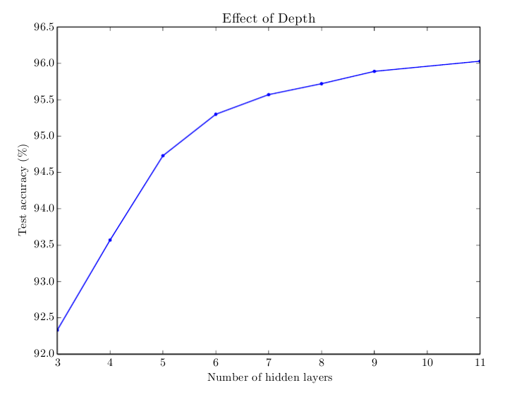
Fig. 2 Relation between the number of layers and accuracy of a model trained to transcribe multi-digit numbers from photographs of addresses by Deep Learning book

The MLP can learn how to approximate functions after a training process where numerous pairs of inputs and expected outputs are presented to the network. The set of all these pairs used for training the network is called training dataset or training set. During the training process, the weights (or parameters) of the network are updated to minimise the error between the predicted output and the expected output. The most widely known and used mechanism to perform this training process is called stochastic gradient descent. There is a full article in this blog about this training process.

Next, let us see how the MLP performs a forward pass using vectorised notation. The input layer (most left-hand side in Fig. 1) takes the data to be processed by the network. We can express the input values of the network as a vector . We can now transform the equation of the computation of a single Perceptron (Eq. 1) in its vectorised version:

(2)

(3)

The subscript refers to the neuron’s index in the layer and the superscript to the index of the layer. The weights vector must have the same length as the input vector (output of the previous layer) and the final activation value is yielded by the activation function . The equation of the computation for the whole layer can be written as follows in the vectorised form:

(4)

(5)

Where is now a two-dimensional matrix with the number of rows equal to the number of neurons in layer and the number of rows equal to the number of neurons in layer , and is a vector of the same size as the neurons in the layer . Finally, if we want to do a forward pass through a dataset with samples we can write Eq. 1 as:

(6)

(7)

In this case, , and are matrices of dimension , has dimensions and the input matrix has dimensions . Where is the dimension of the input and is the dimension of the output for that layer.

When these equations are translated into code run by a program, using the vectorised version instead of loops makes it run much faster. The vector operations can be parallelised taking advantage of the graphic card’s power.

Footnotes

1. That assertion is extracted from Ian Goodfellos et al. book Deep Learning ↩