How the Multi-Layer Perceptron Learns
The learning process of a DNN is formulated as an optimisation problem. It is an iterative method where the parameters of the network are updated to better approximate the function matching the input space to the output space of the dataset. To evaluate how good the prediction of the network is in comparison to the expected value in the training dataset, a loss function is used to provide a score for this approximation. The lower the score, the better the prediction by the network. Therefore, the learning method aims to obtain the parameter values that minimise the result of the loss function, or in other words, find the global minimum of the loss function. In reality, in a multidimensional problem, it is almost impossible to reach this global minimum and reaching a local minimum is a good enough result for the neural network training. The optimisation process consists in backpropagating the gradient of the loss function and updating the weights in the opposite direction of the gradient.
Intuition of gradient descent
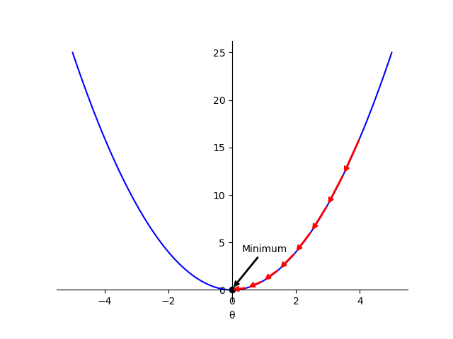
As an intuition on how gradient descent works, we can think of a one-dimensional loss function, for example, the quadratic function

Fig. 1 Intuition for gradient descent with one-dimensional function. The red arrows indicate the leaps during the optimisation process, leading to the global minimum.
Each leap in the figure represents an update in the
The
Cost functions
In the previous paragraphs, we have seen an intuition of how gradient descent works for a network with a single parameter.
Real networks can have thousands of parameters, increasing the dimensionality of the problem.
However, the same principles can be applied, in this case calculating the gradient instead of the derivatives and evaluating the network with a batch of data despite a single point.
When the loss function is calculated for a batch of data it is called cost function (
On the other hand, for classification problems, the output of the network is passed by a softmax (Eq. 3) layer that calculates the normalised vector of classes probabilities and then we apply the cross entropy loss (CE) (Eq. 4) function. This function gives sparse values for different output classes that have similar inputs, which is the main reason why it is preferred over the MSE for classification problems.
Both the CE and MSE loss functions have smooth gradients that are simple to compute, thereby facilitating the training process and its convergence.
Calculating the gradients
As mentioned, the optimization algorithm computes the gradient of the cost function updating the parameters of the network in the process. Continuing with the MLP example, the first step is to do a forward pass to calculate the outputs for a set of inputs following the MLP equations that you can find in this post. Then the result of the loss function is calculated using the outputs of the network and the expected outputs in the dataset. Using the chain rule the gradients are calculated as follows from the cost function:
And the parameters of each layer are updated as follows:
In the example explained above, we have assumed that the dataset contains the expected outputs for the corresponding inputs and the training process is called supervised learning. Most models that we use nowadays are trained using a supervised learning approach. However, due to the difficulty of gathering data for some specific applications, we often do not have labels (or expected outputs) in our dataset. Therefore, there are other learning approaches such as self-supervised learning or reinforcement learning. You can find an example of a project using self-supervised learning in the projects page for training a model for 3D human pose estimation.
Initialisation and normalisation
Before plunging into the optimisation of gradient descent, it is crucial to underscore the importance of correctly initialising the network weights and normalising the input. Regarding the initialisation of the learnable parameters, one possibility is to set all of them to the same value. However, this is not a favourable option, as it results in all neurons performing identical operations and processing the same gradients, therefore leading to the so-called symmetry problem. In such a configuration, the network will not be able to learn and update its parameters, making it useless to have more than one neuron per layer. For this reason, the initial weight values are sampled from a random distribution. However, the choice of the distribution must be done carefully to avoid vanishing/exploding gradient problems or falling into the aforementioned symmetry problem. Gradients vanishing become too small to have any effect and exploding become too large, leading to numerical instability. The selection of the distribution is often based on the number of inputs or fan in, the number of outputs or fan out, the type of activation and the type of network. The three most common initialisation techniques in deep learning are listed here:
- The LeCun initialisation 2 normalises the variance of the sampling distribution to avoid it growing with the number of inputs.
This allows the neurons have a significant output variance.
The weights are drawn i.i.d. with zero mean and a normalised variance with the number of inputs
:
- Xavier initialisation 3 also takes into account the fan out
for a more efficient performance during backpropagation. It works better with sigmoid and hyperbolic tangent activations.
- Finally, He initialisation 4 introduces a slight modification and it works better with ReLU or LeakyReLU activation types.
In practice, all the frameworks utilised throughout this thesis offer a default initialisation for each type of layer. Based on my experience, employing these default initialisations has proven effective, and I have not encountered the need to alter or fine-tune them. For instance, the default initialisation for the weights of a fully connected layer in PyTorch5 is:
Turning now to the normalisation topic, it is also a crucial step before training the network. The normalisation step sets the inputs to have zero mean and the variance to 1, this way all the input variables are in a similar range. The normalisation of the input creates a more symmetric cost function, which helps to stabilise the gradient descent step, allowing us to use larger learning rates or help models converge faster for a given learning rate. Fig. 2 depicts an intuition of how the normalisation can affect the shape of the cost function for a hypothetical network with two parameters. Normalising the input data can also help the model to generalise better to new data. This is because the model is less sensitive to the scale of the input data, and is, therefore, less likely to overfit the training data. Normalised inputs also prevent the problem of exploding and vanishing gradients.
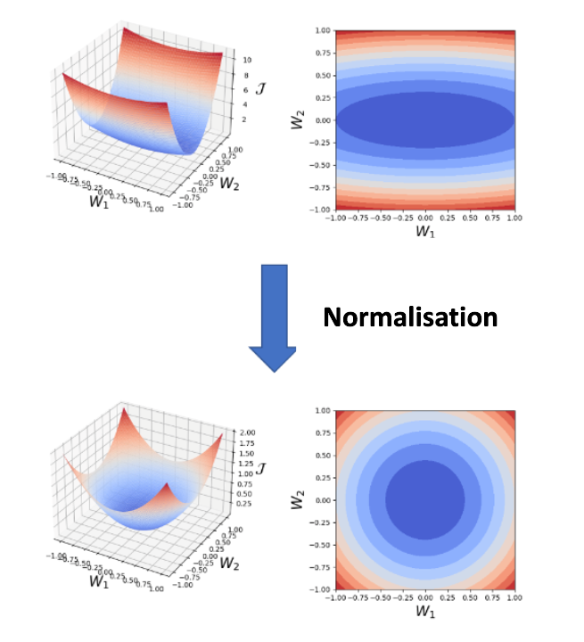
Fig. 2 An illustrative example of how the normalisation of the input can make the loss function more symmetric, which speeds up and stabilise the learning process.
It is important to include in this post the batch normalisation technique6.
It follows similar principles of normalising the input data but in this case, it normalises the activations
After the activation vector is normalised the activations are updated as follows:
Where
There are several benefits to using batch normalisation:
-
Batch normalisation has been shown to significantly improve the performance of neural networks, especially when the network is deep or has a lot of layers6. It speeds up and stabilises the training following the same intuition seen earlier with the normalisation of the input data.
-
In some cases, batch normalisation can reduce the need for dropout, a regularisation technique (explained in this post) used to prevent overfitting since it also adds a slight regularisation effect.
-
Batch normalisation can make it easier to tune the hyperparameters of a neural network, such as the learning rate because it helps to stabilise the activations and gradients. This can make the network more robust to changes in the hyperparameters and allow for more efficient training.
Footnotes
-
Bengio, Yoshua. “Practical recommendations for gradient-based training of deep architectures.” Neural networks: Tricks of the trade: Second edition. Berlin, Heidelberg: Springer Berlin Heidelberg, 2012. 437-478. ↩
-
LeCun, Yann, Léon Bottou, Genevieve B. Orr, and Klaus-Robert Müller. “Efficient backprop.” In Neural networks: Tricks of the trade, pp. 9-50. Berlin, Heidelberg: Springer Berlin Heidelberg, 2002. ↩
-
Glorot, Xavier, and Yoshua Bengio. “Understanding the difficulty of training deep feedforward neural networks.” In Proceedings of the thirteenth international conference on artificial intelligence and statistics, pp. 249-256. JMLR Workshop and Conference Proceedings, 2010. ↩
-
He, Kaiming, Xiangyu Zhang, Shaoqing Ren, and Jian Sun. “Delving deep into rectifiers: Surpassing human-level performance on imagenet classification.” In Proceedings of the IEEE international conference on computer vision, pp. 1026-1034. 2015. ↩
-
Documentation for a fully connected layer in the framework PyTorch: https://pytorch.org/docs/stable/generated/torch.nn.Linear.html. ↩
-
Ioffe, Sergey, and Christian Szegedy. “Batch normalization: Accelerating deep network training by reducing internal covariate shift.” In International conference on machine learning, pp. 448-456. pmlr, 2015. ↩ ↩2